Database Scaling Foundations Every Programmer Should Understand: From Replication to CAP

When a business says:

“The database is slow.”

or:

“We are worried the database will not survive next month’s campaign.”

the conversation changes. It is no longer just about query speed. It is about whether one database can carry the weight of the business at all.

This is where Level 3 of the foundation series begins.

In the previous part, we discussed latency, throughput, caching, indexing, load balancing, CDN, and DNS. Those techniques help us squeeze more performance out of a single system. But at some point, squeezing is no longer enough. We need to spread the data across more machines.

In this part, we will discuss:

• Data Replication
• Read Replicas
• Data Partitioning
• Sharding
• Consistent Hashing
• Denormalization
• Consistency Models
• CAP Theorem

The goal is not to make you a database internals expert. The goal is to help you understand what trade-offs you are taking on when the system stops fitting in one database, and to communicate those trade-offs clearly with the team.

---

1. Why One Database Is No Longer Enough

Before we talk about techniques, let us start with the question: why does one database stop being enough?

There are several common reasons:

• The data volume is too large for a single server’s storage.
• The read traffic is too high for a single server to handle.
• The write traffic is too high for a single server’s CPU or disk.
• A single server becomes a single point of failure.
• The dataset is too big to back up within an acceptable window.
• The geographic distance between users and the database adds too much latency.

When any of these become real, the conversation moves from “make the query faster” to “distribute the data”.

From a System Analyst perspective, the first questions to ask are usually:

• Is the bottleneck CPU, memory, disk I/O, or network?
• Is the workload read-heavy, write-heavy, or balanced?
• Can we tolerate stale data for a few seconds?
• Can we tolerate some downtime during a failover?
• What is the cost of data loss versus the cost of complexity?

Without these answers, scaling the database becomes guesswork.

---

2. Data Replication

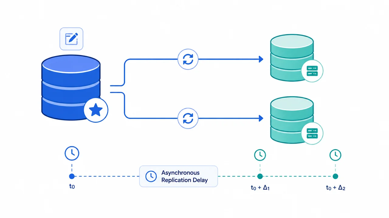
Replication is the act of copying data from one database to one or more other databases.

The typical setup:

                ┌── Replica 1
                │
Primary DB  ────┼── Replica 2
                │
                └── Replica 3

The primary database accepts writes. The replicas receive copies of those writes. Clients can then read from either the primary or the replicas.

Why Replicate

Replication helps with several problems at once:

• Read traffic can be distributed across multiple servers.
• If the primary fails, a replica can be promoted to take over.
• Replicas can be placed closer to users in different regions.
• Backups and analytics can run against replicas instead of the primary.

How Changes Propagate

But replication also raises a question:

When the primary changes a row, when does the replica see the change?

There are two common patterns:

Synchronous replication. The primary waits until at least one replica confirms it has written the change. Only then does the primary acknowledge the write to the client.

Pros:

• Replicas are always up to date.
• No risk of losing the latest write if the primary dies.

Cons:

• Write latency includes the round trip to the replica.
• If the replica is slow, the primary is slow.
• If the replica is unavailable, writes can fail.

Asynchronous replication. The primary writes locally and immediately acknowledges the client. The replica catches up later.

Pros:

• Very fast writes on the primary.
• Replica outage does not block writes.

Cons:

• Replica can lag behind by seconds or minutes.
• If the primary dies before the replica catches up, recent writes can be lost.

Replication Lag

The gap between “data is written on the primary” and “data is visible on the replica” is called replication lag.

This is where many subtle bugs appear:

• A user updates their profile, refreshes the page, and sees the old name.
• An e-commerce system shows that an item is in stock, but the order fails because the primary has already sold the last unit.
• A report generated from a replica shows fewer rows than a report from the primary.

Lag is not a bug. It is a property of asynchronous replication. The question is whether the application is designed to handle it.

From a System Analyst perspective:

“How much lag is acceptable for this feature, and what happens when it is exceeded?”

---

3. Read Replicas

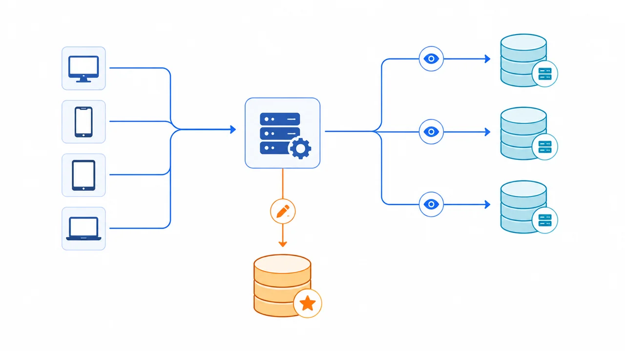
A read replica is a replica that is used primarily for read traffic. The idea is simple: split the database workload so that writes go to the primary, and reads go to the replicas.

                ┌── Read Replica 1
                │
Client ──> App ─┼── Read Replica 2
                │
                └── Primary Database
                     │
                     └── Write

Why It Helps

Many applications are read-heavy. Dashboards, listings, reports, and search pages usually read far more than they write. By spreading reads across replicas, the primary is freed to focus on writes.

Trade-offs

The trade-offs are not free:

• Read queries must tolerate some lag. They may see slightly older data.
• Cross-replica reads (for example, joins across two replicas) are tricky.
• The application must be aware of which connection goes where.
• If one replica lags badly, some reads become slower than others.

When It Works Well

Read replicas work well when:

• The workload is read-heavy.
• Slightly stale data is acceptable (a few seconds is usually fine).
• Reads can be classified clearly as “needs fresh data” versus “eventually consistent is fine”.

When It Does Not Work

Read replicas do not help much when:

• Writes are the bottleneck. Replicas do not reduce write load.
• The data must always be fresh. Strong consistency is required.
• The workload is heavy on multi-row transactions that span many tables. Those usually need to hit the primary anyway.

A common mistake is to assume that adding replicas always helps. If the primary is CPU-bound because of writes, adding replicas only adds cost without relieving the bottleneck.

---

4. Data Partitioning

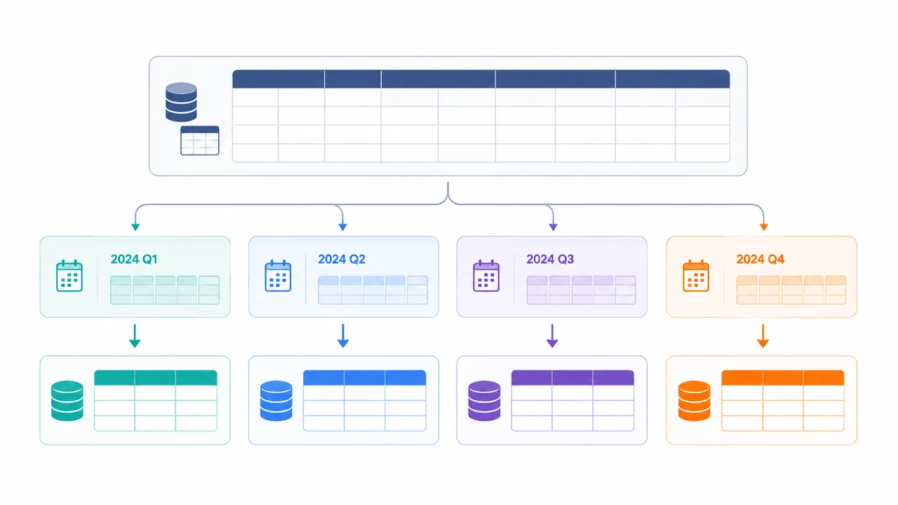
When one table becomes very large, the database itself can split the table into smaller pieces. This is called partitioning.

Partitioning is usually done by the database engine itself. The application still sees one logical table, but the storage is split into separate physical pieces.

Common partition keys:

• Date range: one partition per month or per year.
• Region: one partition per geography.
• Customer segment: one partition per tier.
• Status: one partition for active rows, one for archived rows.

Example in PostgreSQL syntax:

CREATE TABLE orders (
    id BIGINT,
    customer_id BIGINT,
    order_date DATE,
    total_amount DECIMAL(12, 2),
    PRIMARY KEY (id, order_date)
) PARTITION BY RANGE (order_date);

CREATE TABLE orders_2025 PARTITION OF orders
    FOR VALUES FROM ('2025-01-01') TO ('2026-01-01');

CREATE TABLE orders_2026 PARTITION OF orders
    FOR VALUES FROM ('2026-01-01') TO ('2027-01-01');

Why Partitioning Helps

Partitioning helps in several ways:

• Queries that filter by the partition key only scan the relevant partition.
• Old data can be dropped quickly by removing a partition.
• Bulk loads and index maintenance can be done per partition.
• Some operations can run in parallel across partitions.

When Partitioning Hurts

Partitioning is not magic. Common pitfalls:

• Queries without a partition key in the WHERE clause scan every partition.
• Choosing the wrong partition key leads to uneven sizes (one huge partition, many small ones).
• Cross-partition queries become more expensive than expected.
• Joins across many partitions can be slow if the partitioning strategy does not match the query pattern.

The key question is:

“Does our most common query include the partition key in its WHERE clause?”

If the answer is no, partitioning will not help as much as expected.

From a System Analyst perspective, partitioning is often a good first step before considering sharding. It keeps the database as one logical unit, but distributes the physical load.

---

5. Sharding

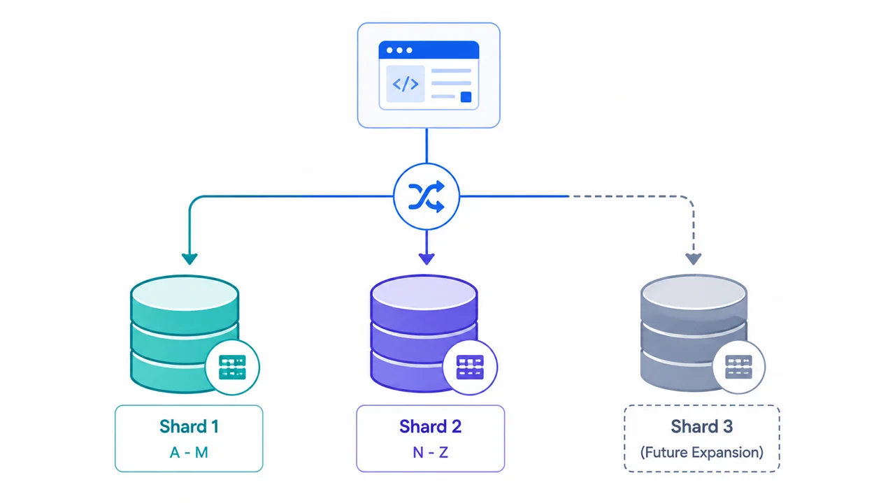
Partitioning splits data within one database. Sharding takes the next step: data is split across multiple independent database servers.

Customer A-M ──> Database Shard 1
Customer N-Z ──> Database Shard 2

Each shard is its own database with its own CPU, memory, and disk. Together, the shards hold all the data.

Why Sharding Helps

• Storage and compute scale horizontally. Add more shards to grow.
• A failure in one shard affects only that shard’s data, not the whole system.
• Writes can be distributed across many servers.

Why Sharding Is Hard

Sharding is one of the most complex decisions in database design. The trade-offs are significant:

• Cross-shard queries become expensive. A query that needs data from two shards must hit both.
• Joins across shards are hard. Some databases do not support them at all.
• Transactions across shards are complex and slow. Two-phase commit and similar protocols add latency and failure modes.
• Rebalancing is painful. When one shard becomes too large, moving data to a new shard is non-trivial.
• Shard key choice is critical. A bad key leads to hot shards where one shard handles most of the traffic.

Choosing a Shard Key

A good shard key:

• Has high cardinality. Many distinct values.
• Distributes data evenly. No single shard becomes too large.
• Aligns with the most common query. Most queries include the shard key, so they hit only one shard.

Common shard keys:

• customer_id for user-centric systems.
• order_id or invoice_id for transactional systems.
• tenant_id in multi-tenant SaaS applications.

A common mistake is to shard by something that does not match query patterns. For example, sharding by created_at for a system that always queries by customer_id forces every query to hit every shard.

Scaling a database often means moving the problem from “limited resource” to “limited simplicity”.

Sharding solves capacity. It also creates operational complexity. A System Analyst should ask whether the business actually needs sharding today, or whether read replicas and partitioning are still enough.

---

6. Consistent Hashing for Data Placement

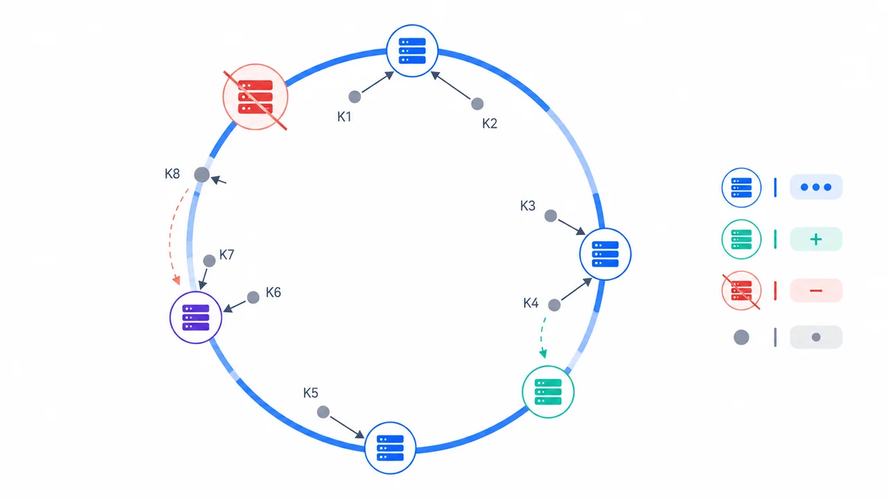
Once we shard, we need to decide: given a key, which shard holds the data?

The simple approach is:

shard = hash(key) % number_of_shards

This works, but it has a problem:

When the number of shards changes, almost every key gets remapped to a different shard.

Imagine we have 4 shards and we add a 5th. The hash modulo changes for almost every key, which means almost every record has to be moved. During the move, the system is under heavy load, and queries for moving records return errors or stale results.

How Consistent Hashing Helps

Consistent hashing solves this by mapping both keys and servers onto the same ring. Each key is assigned to the next server clockwise on the ring.

              Shard A
           ┌─────────┐
       ╱╲  │         │  ╱╲
     ╱    ╲│         │╱    ╲
   ╱   ╱╲  │  Ring   │  ╱╲   ╲
  │   ╱  ╲ │         │ ╱  ╲   │
  │  │ Key│ │         │ │Key │  │
   ╲   ╲ ╱ │         │ ╲ ╱   ╱
     ╲    ╱│         │╲    ╱
       ╲╱  │         │  ╲╱
           └─────────┘
              Shard B

When a new server is added, only the keys between the new server and the previous server clockwise are remapped. The rest of the keys stay where they are.

This is useful because:

• Adding a node affects only a small slice of keys.
• Removing a node affects only that node’s slice.
• Rebalancing is much smoother.

Virtual Nodes

In practice, each physical server is represented by several “virtual nodes” on the ring. This helps distribute load more evenly, because one powerful server can take on multiple slices.

Adding a server should not force the entire dataset to “move house”.

Consistent hashing is used in many distributed systems: caches, key-value stores, message queues, and even some load balancers. In the previous part of this series, we saw consistent hashing as a load balancing algorithm. Here we use it as a data placement strategy. The core idea is the same: minimize remapping when the cluster changes.

---

7. Denormalization

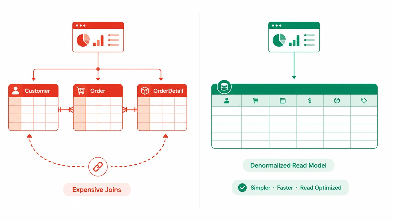
A normalized database is clean. Each fact is stored once. Customer name lives in the customer table. Order details live in the order table. To build a dashboard view, we join them.

Normal:
Customer + Order + Order Detail
        ↓ JOIN
Display Dashboard

The problem is that JOINs become expensive at scale. A dashboard query that joins five tables across millions of rows can be slow even with good indexes.

What Denormalization Does

Denormalization deliberately stores redundant data to make reads faster. The dashboard view becomes its own table or document, pre-joined and ready to read.

Denormalized Read Model
        ↓
Used directly by Dashboard

Example:

-- Normalized view (slow at scale)
SELECT c.name, o.order_date, oi.product_name, oi.quantity
FROM customers c
JOIN orders o ON c.id = o.customer_id
JOIN order_items oi ON o.id = oi.order_id
WHERE c.id = 1001;

-- Denormalized read model (fast)
SELECT customer_name, order_date, product_name, quantity
FROM customer_order_summary
WHERE customer_id = 1001;

The denormalized table is updated by background jobs whenever the underlying data changes.

Trade-offs

Denormalization is a real trade-off:

• Reads become very fast.
• Storage grows because data is duplicated.
• Writes become more complex. Every change to a customer name may need to update many tables.
• Risk of inconsistency. If the background job fails, the read model can be stale.

This pattern is common in read-heavy systems. Search engines, analytics dashboards, and product catalogs often use denormalized views.

When to Use It

Use denormalization when:

• The same heavy query is run many times.
• Slight staleness in the read model is acceptable.
• The team is willing to maintain the synchronization logic.

Avoid denormalization when:

• The data changes too often. Updates become too expensive.
• Strong consistency is required. Denormalized views are eventually consistent by nature.
• The team cannot afford the operational overhead of keeping them in sync.

---

8. Consistency Models

In a distributed database, “the data has been updated” does not always mean:

Every user sees the new value at the same moment.

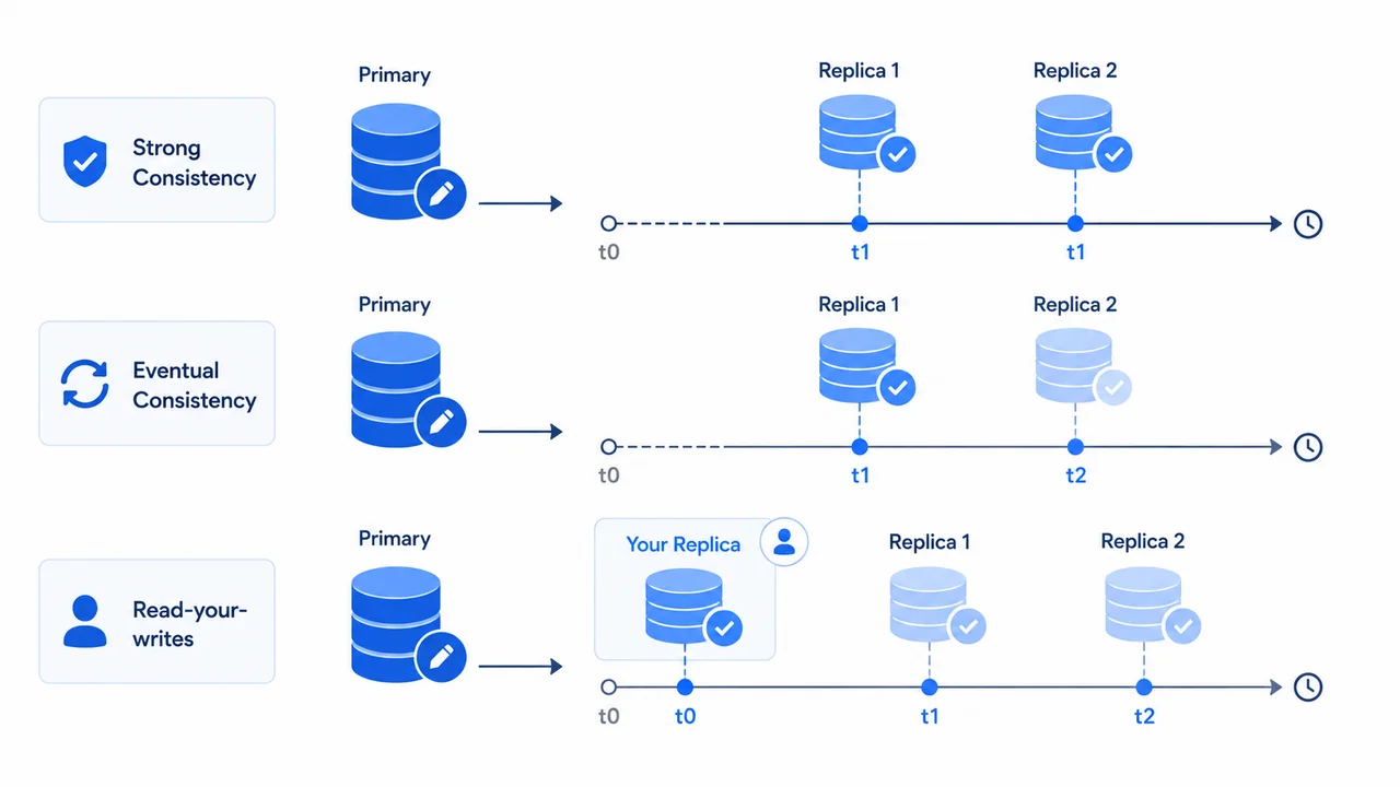
Different systems make different promises about when updates become visible. These promises are called consistency models.

Strong Consistency

After a write completes, every subsequent read sees that write (or a newer one).

Use case:

• Banking systems. A transfer must be visible immediately.
• Inventory systems where overselling must be prevented.

Trade-off:

• Higher write latency.
• Lower availability during network problems.

Eventual Consistency

If no new updates are made to a piece of data, eventually all replicas will converge to the same value. But there is no guarantee about when.

Use case:

• Social media feeds.
• Product catalogs.
• View counters.

Trade-off:

• Very high availability and performance.
• Users may see older data for a while.

Read-Your-Writes Consistency

After a user writes a value, that user’s own subsequent reads always see the write. Other users may still see older values until replication catches up.

Use case:

• A user updates their profile picture and refreshes the page. They should see their new photo, even if their friends still see the old one.

Trade-off:

• Easier to reason about for the user who made the change.
• Still eventually consistent for other users.

Causal Consistency

Operations that are causally related are seen by all nodes in the same order. Unrelated operations may be seen in different orders.

Use case:

• Comment threads. Replies must appear after the original comment, but unrelated comments can appear in any order.

Why This Matters

A common confusing experience:

“I just updated my balance. I refreshed the page. The old balance is still there.”

Is the system broken? Not necessarily. It might just be replication lag or eventual consistency.

From a System Analyst perspective:

“What consistency guarantee does this feature need, and what consistency guarantee does the chosen database provide?”

If the answer does not match, the system will behave strangely at some point.

---

9. CAP Theorem

The CAP theorem is one of the most cited and most misunderstood ideas in distributed systems. It says:

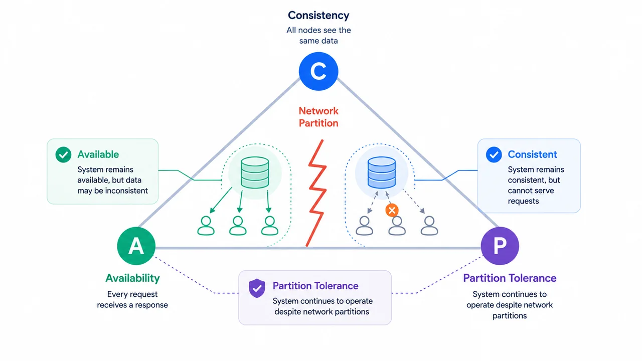
In a distributed data store, when a network partition happens, you must choose between Consistency and Availability.

Let us break that down.

The Three Properties

• Consistency (C). Every read sees the latest committed write, or an error.
• Availability (A). Every request receives a response (non-error), even if it cannot guarantee the latest data.
• Partition tolerance (P). The system continues to operate despite network failures between nodes.

The Common Misunderstanding

Many introductions say:

“Pick two out of three.”

This is misleading. In a distributed system, network partitions will happen. P is not a choice. P is a given. So the real question is:

“When a partition occurs, do we prioritize C or A?”

Consistency During Partition (CP)

The system refuses writes (or reads) on the side of the partition that cannot reach the latest data. It would rather return an error than give a possibly wrong answer.

Examples:

• Traditional relational databases configured for synchronous replication.
• Some distributed databases that favor strong consistency.

Availability During Partition (AP)

The system continues to accept reads and writes on both sides of the partition. Each side works with the data it has. When the partition heals, the system reconciles.

Examples:

• DNS.
• Most eventually consistent key-value stores.
• Many NoSQL databases.

What CAP Does Not Cover

CAP is about what happens during a partition. It does not cover:

• Normal operation latency.
• Performance under load.
• Cost of reconciliation after a partition.
• How long a partition can last before consistency is restored.

CAP is not a feature checklist. It is a way to think about trade-offs when the network fails.

From a System Analyst perspective, the question is not “are we CP or AP?” but “for each service in our system, what is the right trade-off?”.

A banking ledger is usually CP. A product catalog is usually AP. A session store might be AP with read-your-writes. The right answer depends on the business requirement, not on the database marketing page.

---

10. Putting It All Together: A Simple Example

Let us put these concepts into one example.

Requirement:

“User opens the order history page.”

Step by step:

Replication

1. The order service writes new orders to the primary database.
2. The change is replicated asynchronously to two read replicas.

Read Replica Routing

1. The order history request is identified as a read.
2. The application routes it to one of the read replicas.

Partitioning and Sharding

1. The orders table is partitioned by order_date (one partition per quarter).
2. Orders are sharded by customer_id across four shards.
3. The router computes the shard from the user ID and sends the query there.

Consistent Hashing

1. The shard router uses consistent hashing so adding a fifth shard in the future will not remap every customer.

Denormalized Read Model

1. A background job listens to changes in the normalized tables.
2. It maintains a denormalized customer_order_summary view, pre-joined and ready to read.
3. The order history page reads from the read model, not from the live tables.

Consistency Model

1. The read model is eventually consistent. A user who just placed an order may see it missing for a few seconds.
2. The order detail page forces a read from the primary to avoid that lag.

CAP Behavior

1. If the network between regions partitions, the read replicas in the affected region continue serving slightly older data (AP behavior).
2. The order placement endpoint refuses writes if it cannot reach the primary (CP behavior).

Now imagine a problem at each step:

Problem	Symptom
Replication lag too high	Users see outdated order status
Read replica overloaded	Slow order history page
Bad shard key	One shard becomes a hot spot
Denormalized job failed	Read model returns empty or stale data
Wrong consistency model	User sees their order missing right after placing it
Network partition ignored	Users see conflicting data across regions

The point is: database scaling is rarely fixed by one technique. It is a combination of replication, sharding, caching, and consistency decisions.

---

11. Common Mistakes

These mistakes appear often in real projects.

Sharding Too Early

Sharding adds enormous complexity. Many systems that sharded at 10 GB of data never needed to. Read replicas and partitioning would have been enough.

Choosing the Wrong Shard Key

A shard key that creates hot spots is worse than no sharding at all. One shard takes most of the traffic, and the others sit idle.

Ignoring Replication Lag

Treating a replica as if it always has the latest data. The application behaves correctly most of the time, then breaks under load when lag grows.

Denormalizing Without a Sync Strategy

Copying data into a read model without a clear plan for keeping it in sync. The read model drifts, and eventually users notice.

Assuming CAP Means “Pick Two”

Treating CAP as a checklist rather than a trade-off during network partitions. Picking the wrong trade-off for the wrong feature.

Forgetting About Rebalancing

Designing a sharding scheme that works today but cannot be rebalanced when one shard grows. The team is stuck with an uneven system.

Skipping Observability

Without metrics on replication lag, shard distribution, and consistency violations, problems become invisible until users complain.

Optimizing for One Query Type

Designing the shard key for the most common query, then realizing later that reporting and analytics need a different access pattern.

---

12. How a System Analyst Reads Database Requirements

When a requirement mentions database scaling, a System Analyst can use this checklist:

Workload

• Is the system read-heavy, write-heavy, or balanced?
• What is the current and projected data volume?
• What is the current and projected QPS?

Consistency

• Does this feature need strong consistency?
• Is eventual consistency acceptable? For how long?
• Are there features where the user must see their own writes immediately?

Availability

• What is the cost of downtime for this service?
• Is multi-region deployment required?
• What is the recovery time objective (RTO) and recovery point objective (RPO)?

Distribution

• Where are the users geographically?
• Do we need replicas in multiple regions?
• Can we tolerate cross-region latency?

Sharding Strategy

• What is the natural access pattern? By user, by tenant, by date?
• What is the cardinality of the shard key?
• Can we rebalance without a major outage?

Read Model

• Are there queries that are too heavy even with indexes?
• Is denormalization acceptable?
• Who maintains the read model?

Observability

• Can we measure replication lag?
• Can we measure per-shard QPS?
• Do we have alerts for consistency violations?

These questions turn a vague “scale the database” request into a set of concrete design decisions.

---

13. Closing

Database scaling is not a single technique. It is a set of decisions that interact with each other:

• Replication decides how many copies of the data exist.
• Read replicas decide how read traffic is distributed.
• Partitioning decides how data is split within a database.
• Sharding decides how data is split across databases.
• Consistent hashing decides where each key lives.
• Denormalization decides how much we trade storage for read speed.
• Consistency models decide what users see and when.
• CAP reminds us that during network partitions, every system makes a trade-off.

When we discuss a database scaling requirement, we should not jump to a solution. We should ask:

“Which part of the workload is the bottleneck, how fresh does the data need to be, and which trade-offs are we willing to accept?”

Performance work, application work, and database work are all connected. The deeper we go, the more important it becomes to see the system as a whole.

---

Related Articles

• Performance Scaling Foundations Every Programmer Should Understand: From Latency to DNS
• Fondasi Performa dan Scaling yang Perlu Dipahami Programmer: Dari Latency ke DNS (Indonesian version)
• Web and API Foundations Every Programmer Should Understand: From Client-Server to JWT
• Fondasi Web dan API yang Perlu Dipahami Programmer: Dari Client-Server ke JWT (Indonesian version)